This article is a summary of the 6th assignment for the Fall 2018 Computational Linguistics course, with the task of generating adversarial input sequences based on RNN.

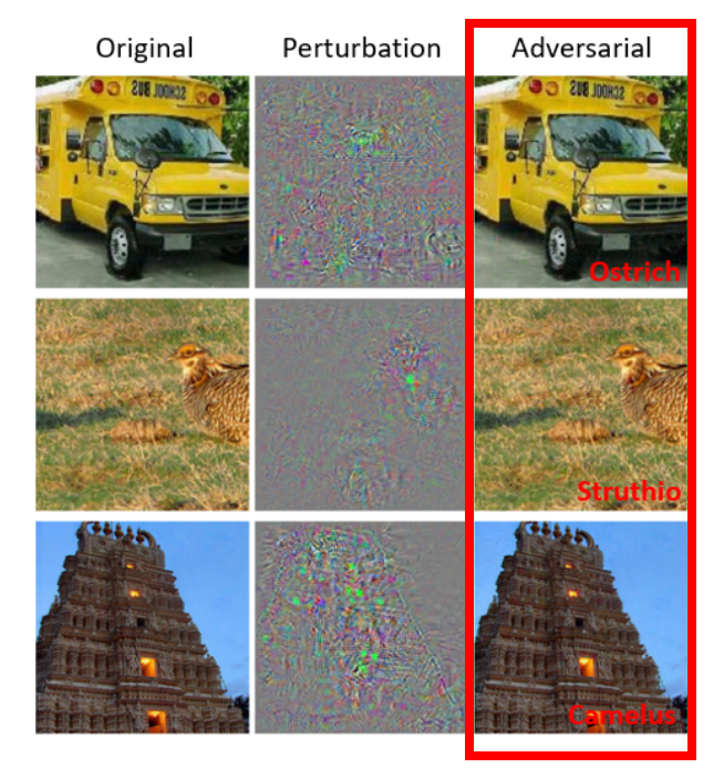
First, let me give an overall introduction to the concept of adversarial example attacks. Some researchers have found that although deep neural networks achieve very high accuracy, applying small perturbations to the input can cause the model's prediction results to be completely wrong. For images, such perturbations are usually so subtle that they are imperceptible (humans cannot intuitively perceive the perturbation in the image), yet these adversarial input examples can successfully fool deep learning models. This type of attack that deceives neural network models can be broadly divided into two categories: untargeted attacks only need to make the predicted result of the image inconsistent with the original label, while targeted attacks need to misclassify the image as a specific class. It is worth noting that researchers have found that generated adversarial examples are still effective on other models, which is known as the transferability of adversarial examples.

The results shown here are mainly adversarial examples generated on convolutional neural networks (CNNs):

cnn_adversarial_example

Generating Adversarial Input Sequences for a PTB Language Model

Model Preparation

First, I tried to run the language model training code provided by TensorFlow. After running it, I found that this code only prints the model's perplexity and does not provide an interface to input a sentence/a word and predict the next word. Therefore, I also referenced the version modified by Rani Nelken on GitHub based on the PTB language model training code. The differences are:

Established bidirectional mapping between numeric IDs and word IDs
Fine-tuned the RNN structure, mainly modifying the process from the RNN output to the loss computation, retaining the intermediate results logits to obtain the probabilities for the next word prediction
Modified the file reading code so that each iteration returns the previous word x and the next word y from the test text

Using Rani Nelken's version of the code, after 13 epochs of training with the small parameters, the language model weights usable for testing were obtained.

Approach for Generating Adversarial Input Sequences

Here, I mimic the FGSM method to generate adversarial input sequences. First, let me give a brief introduction to the FGSM method [1]: The FGSM method is an approach for computing adversarial perturbations proposed by Ian Goodfellow et al. in 2015. FGSM exploits the "linear" property of deep network models in high-dimensional space (while such models are typically considered highly nonlinear) to efficiently generate large numbers of adversarial examples. The formula for computing perturbations using the Fast Gradient Sign Method (FGSM) is as follows:

$p = \epsilon sign(\nabla J(\theta,I_c,l))$

Where $I_c$ represents the original image, $l$ is the label of the misclassified category, $\theta$ is the neural network parameters, $\nabla J$ denotes the gradient of the cost function with respect to the network model parameters $\theta$ computed on the current original image $I_c$ , and $sign$ is the sign function (turning the originally nonlinear perturbation into a linear perturbation), defined as follows:

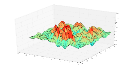
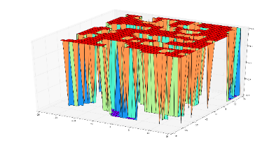
sign(x) = \begin{cases} 1, & x>0 \\ 0, & x=0 \\ -1, & x<0 \\ \end{cases}

The role of $\epsilon$ is to constrain the strength of the perturbation to be as small as possible. The two figures below intuitively show examples of the original gradient and the gradient after the sign function is applied, respectively.

Original Gradient	Gradient After Sign Function

During the execution of the language model, the formula for computing the perturbation p is as follows:

$p = \epsilon \nabla J(\theta,I_c,l)$

Where $I_c$ represents the embedding corresponding to the original input sequence, $l$ is the label classified from the final state output of the RNN after computing logits, $\theta$ is the neural network parameters, $\nabla J$ denotes the gradient of the cost function with respect to the network model parameters $\theta$ computed on the embedding $I_c$ corresponding to the current input sequence, and $\epsilon$ is the perturbation magnitude that can be manually controlled.

The reason for not using the sign function $sign$ here is mainly that the magnitude of the perturbation (approximately $10^{-3}$ ~ $10^{-2}$ ) is smaller than the magnitude of the embedding (approximately $10^{-1}$ ). Therefore, if the sign function $sign$ is used, the resulting perturbation embedding would be too large, leading to a large computed distance, which deviates significantly from the goal of a "small" perturbation.

Since the input sequence to the RNN language model is discrete — i.e., the input words, after being converted to numeric IDs, are further converted into vectors through an embedding layer before participating in the RNN computation — even if the perturbation p is directly added to the original embedding $I_c$ , there is a high probability that the embedding still cannot be directly converted to a word ID. Therefore, the approach here is to compute the nearest Euclidean distance to convert the perturbed embedding into the word ID of the nearest embedding, thereby changing the input sequence. The process is as follows, where $e$ represents the embedding corresponding to the original word ID, $p$ represents the perturbation, and $e^*$ represents the embedding after adding the perturbation:

$e^* = e + p$

Then, solve for the embedding ID nearest to the perturbed embedding $e^*$ , where n is the number of words in the corpus; in this experiment, n=20000:

$argmin_{id}{\sqrt{\sum_{id=0}^{n}(e^{*}-e_{id})^2}}$

Results of Adversarial Input Sequence Generation

Example of Adversarial Input Sequence

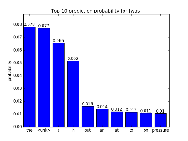
The original test input sequence used here is {no it was n't}. We generate an adversarial input sequence for the second-to-last word was. By adding the computed perturbation, the adversarial sequence obtained is {no it being n't}. This allows us to observe the change in the prediction probabilities of the next word for the second-to-last word.

Visualization of the Probability Distribution for Predicting the Next Word

Next Word Prediction Probabilities for "was"	Next Word Prediction Probabilities for "being"

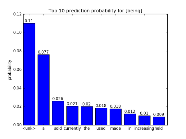It can be seen that the Top 10 probability distribution of the next word prediction for the adversarial sequence has changed, especially the Top 1 predicted word, which changed from the to <unk>. There are still some shortcomings in this experiment, such as the lack of quantitative metrics (e.g., perplexity, etc.) to evaluate the quality of the generated adversarial input sequences. In the future, adding adversarial sequences to the retraining process of the language model could be considered.

Generating Adversarial Input Sequences for a seq2seq Language Correction Model

Model Preparation

The language correction model used here is based on the open-source code by David Currie on GitHub, which mainly adopts an encoder-decoder network structure based on seq2seq, and also uses attention and bidirectional LSTM structures. Its purpose is to train a language correction model for English corpora. Examples are shown below:

Original sequence: Spellin is difficult, whch is wyh you need to study everyday. Corrected sequence: Spelling is difficult, which is why you need to study everyday.

Original sequence: The first days of her existence in th country were vrey hard for Dolly. Corrected sequence: The first days of her existence in the country were very hard for Dolly.

Using David Currie's code, after adjusting several parameters and training, the model weights for generating adversarial input sequences for the language correction model were obtained. Due to training parameters and other factors, the actual correction effect is not as good as demonstrated by the author, and there are still cases where some words are not corrected; however, this does not affect this experiment.

Approach for Generating Adversarial Input Sequences

Here, I mimic the DeepFool method to generate adversarial input sequences. First, let me give a brief introduction to the DeepFool method [2]: Given a classifier model f, Moosavi-Dezfooli et al. first defined the minimal perturbation r for an image that causes its classification result k to be incorrect, as shown in the following equation:

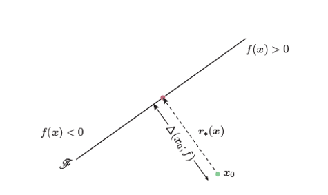
$\Delta(x, \hat{k}) = min_r||r||_2, s.t.\ \hat{k}(x+r) \ne \hat{k}(x)$

After giving the above definition, Moosavi-Dezfooli proposed the DeepFool model: iteratively computing the optimal perturbation direction for a given image, in which direction large numbers of adversarial examples can be generated quickly and effectively. Viewed from the perspective of a simple binary classification model, the direction for generating adversarial examples is illustrated in the figures below:

Adversarial Example Direction for Binary Classification	Adversarial Example Direction for Multi-class Classification

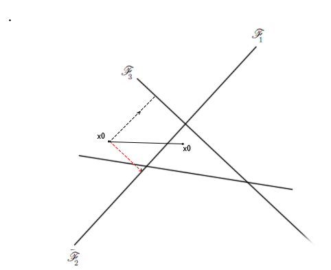Both FGSM and DeepFool aim to make the model predict an incorrect classification, so they need to mutate the original image $x_0$ so that it moves in the direction of misclassification — that is, the direction of gradient ascent to mutate (the dashed arrow direction). On binary classification models, DeepFool and FGSM do not differ in the perturbation direction. However, on multi-class problems, they differ significantly, as illustrated in the figure above.

In this simple three-class classification problem, assume the original image $x_0$ is classified by the model as $y_1$ . To make the classification incorrect, the FGSM model will mutate by adding a perturbation in the direction of the $y_1$ misclassification — the direction of the red arrow in the figure.

The DeepFool method, on the other hand, argues that moving $x_0$ to the triangular region in the figure would greatly increase the probability of misclassification. Therefore, based on this assumption, DeepFool simultaneously computes the gradient of the Top 1 classification result and the gradient of the Top 2 classification result, and adds these two gradients as vectors to obtain the direction in which to add perturbation to the image — that is, the black solid line represents the mutation direction of the original image $x_0$ .

During the execution of the language correction model, the formula for computing the perturbation p is as follows:

$p = \epsilon \nabla J(\theta,I_c,\sum_{i=1}^4l_i - l_0)$

Where $I_c$ represents the embedding corresponding to the original input sequence, $l_0$ is the Top 1 classification label computed from the output of a randomly selected letter in the predicted sequence of the RNN final state after computing logits, $\sum_{i=1}^4l_i$ is the vector sum of the Top 2 ~ Top 5 classification labels, $\theta$ is the neural network parameters, $\nabla J$ denotes the gradient of the cost function with respect to the network model parameters $\theta$ computed on the embedding $I_c$ corresponding to the current input sequence, and $\epsilon$ is the perturbation magnitude that can be manually controlled.

The reason for not using the sign function here is also mainly that the magnitude of the perturbation (approximately $10^{-3}$ ~ $10^{-2}$ ) is smaller than the magnitude of the embedding (approximately $10^{-1}$ ). Therefore, if the sign function $sign$ is used, the resulting perturbation embedding would be too large, leading to a large computed distance, which deviates significantly from the goal of a "small" perturbation.

$e^* = e + p$

Then, solve for the embedding ID nearest to the perturbed embedding $e^*$ , where n is the number of words in the corpus; in this experiment, n=79:

$argmin_{id}{\sqrt{\sum_{id=0}^{n}(e^{*}-e_{id})^2}}$

Results of Adversarial Input Sequence Generation

Example of Adversarial Input Sequence

The original test input sequence used here is

Spellin is difficult, whch is wyh you need to study everyday.

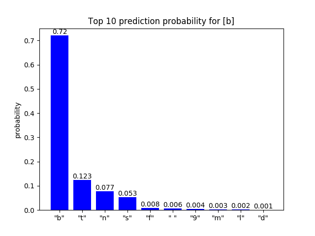
We generate an adversarial input sequence for the 36th character o. By adding the computed perturbation to the embeddings of each possible input character, we obtain a certain adversarial sequence:

Spellin ib difficult, whch is wyh you need to study everyday.

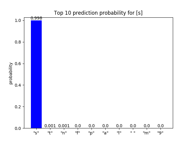
The difference between these two sequences is that the s in is is replaced by b, which allows us to observe the change in the prediction probabilities of the correction character at the corresponding position before and after the replacement.

Visualization of the Probability Distribution for Predicting the Corrected Character

It can be seen that the Top 10 probability distribution of the character prediction at the corresponding position in the adversarial sequence has changed, especially the Top 1 predicted character, which changed from s to b. From the correction results, ib was not corrected to is.

Correction Character Prediction Probabilities for "s"	Correction Character Prediction Probabilities for "b"

There are still some shortcomings in this experiment, such as the lack of quantitative metrics (e.g., perplexity or BLEU, etc.) to evaluate the quality of the adversarial input sequences generated for the language correction model. In addition, the adversarial sequences generated by this method are limited to replacing a single character, and strategies for insertion or deletion have not yet been implemented. In the future, adding adversarial sequences to the retraining process of the language correction model could be considered.

References

[1] Goodfellow, I. J., Shlens, J., & Szegedy, C. Explaining and harnessing adversarial examples (2014). arXiv preprint arXiv:1412.6572. [2] Moosavi-Dezfooli, S. M., Fawzi, A., & Frossard, P. (2016). Deepfool: a simple and accurate method to fool deep neural networks. In Proceedings of the IEEE Conference on Computer Vision and Pattern Recognition (pp. 2574-2582).