Data Mining and Knowledge Discovery on KKBOX Music Data
KKBOX is a leading music streaming service in Asia, boasting the world's most comprehensive collection of Asian pop music. This paper conducts a data mining analysis on the music dataset that KKBOX has provided to the Kaggle community. Through initial cleaning and analysis of the dataset, we propose four data mining–related questions: correlation analysis among features in the dataset, song clustering, user clustering, and predicting whether a user will listen to a particular song repeatedly within a month. We then select appropriate algorithms—such as the K-prototypes clustering algorithm, the t-SNE high-dimensional data visualization algorithm, and the LightGBM algorithm—to address these data mining problems, and finally present corresponding conclusions. In doing so, we explore the application of data mining algorithms to a real-world dataset, transforming knowledge from the data mining classroom into truly practical technology.
Introduction
This paper uses four tables from the music dataset provided by KKBOX to the Kaggle community—members.csv, songs.csv, song_extra_info.csv, and train.csv—and proposes four data mining problems, using them as a guide for analyzing the KKBOX dataset. The four problems are:
-
Correlation analysis among features in the dataset The groups of features in the dataset have intrinsic associations, so analyzing the correlations among feature values helps us better understand the latent connections within the data and extract important features that are useful for predicting users' listening habits.
-
User clustering Performing clustering analysis on music listeners aims to identify similar users, which helps KKBOX better position its user segments.
-
Song clustering Clustering analysis on songs is useful for measuring the similarity among songs, grouping similar songs into approximate clusters, thereby identifying the categories of massive song collections and helping listeners find music they enjoy more quickly.
-
Predicting user listening behavior By predicting whether a user will repeatedly listen to a particular song within a month, we can better recommend songs to listeners and provide more personalized music services.
The structure of this paper is as follows: Chapter 1 is the introduction, outlining the tasks and the paper's structure; Chapter 2 introduces related methods; Chapters 3 through 6 describe the process and results for the four data mining problems; and Chapter 7 presents the summary and reflections on this experiment.
Related Methods
Pearson Correlation Coefficient
In the natural sciences, the Pearson correlation coefficient is widely used to measure the degree of correlation between two variables. The Pearson correlation coefficient between two variables is defined as the quotient of their covariance and the product of their standard deviations:
As the formula shows, the Pearson correlation coefficient is obtained by dividing the covariance by the standard deviations of the two variables. Covariance can reflect the degree of correlation between two random variables: a covariance greater than 0 indicates a positive correlation, while a value less than 0 indicates a negative correlation.
K-prototypes Clustering Algorithm
The K-prototypes algorithm, proposed by Huang [1] and others, is an effective algorithm for clustering data with mixed numeric and categorical attributes. It combines the K-means and K-modes algorithms and introduces a parameter y to control the weight of numeric and categorical attributes during the clustering process. The K-prototypes algorithm mainly consists of four steps:
- Randomly select k data objects from the dataset as initial cluster centers
- Compute the distance from each data object to each cluster center, assign it to the nearest cluster, and update the cluster centers after each assignment
- Once all objects have been assigned to clusters, recalculate the distances of the data objects to the current cluster centers and reassign each object to the cluster whose center is nearest
- Repeat step 3 until the data objects in each cluster stabilize
t-SNE Algorithm
The t-SNE (t-Distributed Stochastic Neighbor Embedding) algorithm [3] is an improved version of the SNE algorithm [2]. By applying t-SNE, the intrinsic structure of high-dimensional data can be revealed by projecting it into a low-dimensional space, uncovering the data's inherent classification characteristics. SNE maps data points onto probability distributions through affine transformation and mainly consists of two steps:
- SNE constructs a probability distribution over pairs of high-dimensional objects, such that similar objects have a higher probability of being chosen, while dissimilar objects have a lower probability of being chosen
- SNE constructs a probability distribution over the points in the low-dimensional space such that the two probability distributions are as similar as possible. By performing dimensionality reduction visualization on the high-dimensional information of clustering results, high-dimensional clustering outcomes can be conveniently observed and analyzed.
LightGBM Algorithm
LightGBM is a distributed gradient boosting framework based on decision tree algorithms. LightGBM addresses the efficiency and scalability problems of traditional GBDT (Gradient Boosting Decision Tree) algorithms on high-dimensional data by employing the following methods: histogram-based decision tree algorithms; a leaf-wise tree growth strategy with depth limits; histogram-based difference acceleration; direct support for categorical features; cache hit-rate optimization; histogram-based sparse feature optimization; and multi-threaded optimization. Ke [4] et al. proposed LightGBM to implement GBDM, which accelerates the traditional GBDT training process by more than 20 times while achieving nearly the same accuracy.
Correlation Analysis Among Features in the Dataset
Data Processing
We select train.csv as the data source. First, we filter, clean, and quantify this dataset—for example, counting the number of musical genres and the number of songwriters and composers; performing one-hot encoding on attributes such as language, system_tab, screen_name, source_type, and year; performing a simple binary classification on song length; and additionally conducting data cleaning, missing value imputation, and outlier handling.
Correlation Analysis Experiment
After processing, we obtained 23-dimensional features. Using the correlation analysis functions in Python's Pandas library and the Pearson correlation coefficient, we computed the pairwise correlations across all dimensions. The experimental results are shown in the figure below:
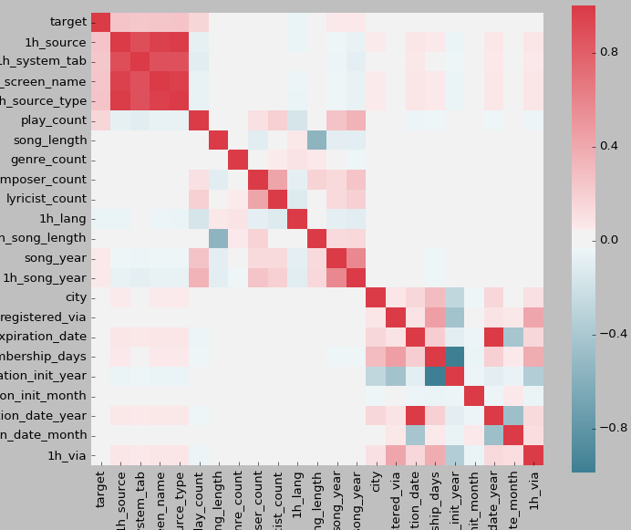
From the experimental results, the following conclusion can be drawn: the variables 1h_source, 1h_system_tab, 1h_screen_name, and 1h_source_type exhibit high correlations with each other, while the other dimensions show lower correlations. 1h_source refers to repeat-play probability; 1h_system_tab refers to the channel that triggered the repeat-play event; 1h_screen_name refers to the page where the repeat-play event was triggered; 1h_source_type refers to the source of the repeat-play event; "1h" indicates that one-hot encoding has been applied to these fields. The listening channel, listening page, and song source are strongly associated in practice. For example, a user's repeat-playing may occur through a search channel on the search page, listening to an online song list. Therefore, under normal circumstances, the search channel, search page, and online song list often co-occur. Moreover, these three attributes all describe the repeat-play behavior, so they each have a strong correlation with the repeat-play rate.
User Clustering
Data Processing
We processed the raw data from the two datasets, members.csv and train.csv, by extracting the year/month/day of registration and cancellation times, membership duration, the total number of songs played by the user, the total number of repeat-played songs, and the repeat-play rate, and handling missing gender attributes (male - 0, missing - 1, female - 2).
User Clustering Experiment
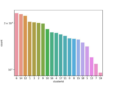
Because the dataset contains discrete attributes such as user IDs and user names, we applied the K-prototypes algorithm to perform K-means clustering (k = 20) on the processed user data, running the clustering process for 100 iterations. After obtaining the clustering results, we performed preliminary statistics on the 20 clusters, as shown in Figure 2:
| Figure 2 Statistics of Records Within User Clusters | Figure 3 t-SNE Visualization of User Clusters |
|---|---|
 |
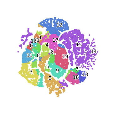 |
As shown in Figure 2, the largest cluster contains more than 2,000 points, while the smallest cluster contains only a few hundred points; overall, the distribution is relatively even. Because the clustering results are high-dimensional data, we used the t-SNE algorithm for dimensionality reduction visualization to analyze the clustering outcomes, as shown in Figure 3. Generally speaking, the higher the density with which data points aggregate within a cluster and the closer they are to the center point, the better the overall quality of that cluster. From Figure 3, we can see that points of the same category mostly appear in clusters, indicating that users within the same category have high similarity.
Song Clustering
Data Processing
Similar to the user clustering process, we processed the raw data from the two datasets, songs.csv, and train.csv, by extracting song release year, genre count, number of singers, number of lyricists, number of composers, the number of times each song was played, and the number of times each song was repeat-played. For missing song years, we imputed using the mode of the year values.
Song Clustering Experiment
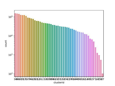
Likewise, because the dataset contains discrete attributes such as song IDs and singer names, we applied the K-prototypes algorithm to perform K-means clustering (k = 50) on the processed song data, running the clustering process for 200 iterations. After obtaining the clustering results, we performed preliminary statistics on the 50 clusters, as shown in Figure 4:
| Figure 4 Statistics of Records Within Song Clusters | Figure 5 t-SNE Visualization of Song Clusters |
|---|---|
 |
 |
As shown in Figure 4, the largest cluster contains more than 100,000 points, while the smallest cluster contains around 100 points; overall, the distribution is relatively even.
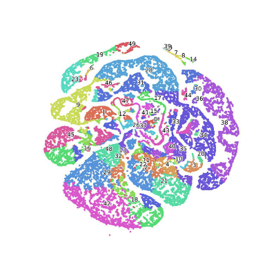
Similarly, we used the t-SNE algorithm for dimensionality reduction visualization to analyze the clustering outcomes, as shown in Figure 5. In Figure 5, songs belonging to the same class are labeled with the same color; there are 50 classes in total. From the figure, we can observe that points of the same category mostly appear in clusters, indicating that songs within the same category have high similarity.
Taking the clustering results of two Jay Chou songs as an example:
| Clustering Result |
|---|
| 253492,465,周杰倫 (Jay Chou),周杰倫,方文山,3.0,園遊會,TWK970400709,6 |
| 166661,458,周杰倫 (Jay Chou),周杰倫,方文山,3.0,公公偏頭痛,TWK971601115,6 |
Both songs are collaborations between Jay Chou and Vincent Fang, with similar musical styles. Our clustering approach successfully grouped them into Cluster 6. This also serves as evidence to some extent that our clustering performance is quite good. Therefore, through this clustering method, we can group similar songs together and then, based on a user's listening habits, recommend similar songs (within the same cluster) in a targeted manner to that user.
Predicting User Listening Behavior
Data Processing
We use the data processing results obtained from the correlation analysis in Section 3.1.
LightGBM Training
Using the LightGBM model and the training set described above, we employed 10-fold cross-validation during the training process for our experiments. Specifically, we divided the training set into 10 subsets; in each round, 9 subsets were used for training and 1 for validation. For each round, we computed the AUC value, and the average of the 10 results was taken as the overall AUC value. The AUC value ranges from 0 to 1 and represents the area under the ROC curve. As a numerical value, AUC provides an intuitive evaluation of classifier performance—the larger the value, the better.
| Experiment Number | AUC |
|---|---|
| 1 | 0.802 |
| 2 | 0.801 |
| 3 | 0.802 |
| 4 | 0.801 |
| 5 | 0.802 |
| 6 | 0.800 |
| 7 | 0.788 |
| 8 | 0.775 |
| 9 | 0.775 |
| 10 | 0.771 |
The average AUC across the 10 experiments is 0.792. From the obtained model, we analyzed the influence of different features on the model: the higher the feature importance, the more important the feature is. To compute feature importance, we first normalize all feature values and then use the "average accuracy reduction" algorithm. The basic idea of this method is to randomly permute the values of a given feature and measure the decrease in accuracy on out-of-bag (OOB) data. If accuracy drops, then the feature is not important; otherwise, it is important. Finally, the degree of influence of each feature is shown in Figure 6:
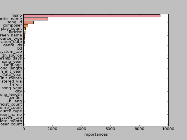
As can be seen from Figure 6, apart from user ID, the song's singer, lyricist, composer, play count, and user play channel have a significant influence on user listening behavior. Therefore, we can draw the following conclusions from the figure above:
- For a given song, whether it will be repeatedly played within a month depends largely on its singer, lyricist, and composer—these are the key factors—while the other features have relatively little influence on the song.
- For a given user, whether the user will repeatedly play a particular song is not strongly related to basic personal information such as age and gender, but is most strongly associated with the user ID, indicating that individual differences in listening habits are enormous and can be viewed as a purely random process. This also suggests, indirectly, that analyzing a user's listening preferences should focus primarily on the user's listening behavioral habits rather than on the user's basic personal information.
Summary and Reflections
Using the pandas data analysis tool, the K-prototypes clustering algorithm, the t-SNE dimensionality reduction visualization algorithm, and the LightGBM model, we conducted a preliminary analysis of four problems on the existing dataset and obtained some preliminary results. However, the results are not ideal; for example, the average AUC value from the LightGBM prediction is below 0.8. The possible reasons for this and areas for improvement include the following:
- The data processing for missing values was relatively crude
- For the two clustering tasks, experiments were only performed with cluster numbers k = 20, 30, and 50. Additional values of k were not tested, and better clustering performance might be obtained with other values of k
- The handling of discrete variables during clustering was inadequate and they should be properly quantified as much as possible
- The clustering results were not effectively integrated with the LightGBM model
References
[1] Huang ZX, Michael KN. A fuzzy k-modes algorithm for clustering categorical data. IEEE Trans. on Fuzzy System, 1999, 7(4): 446–452 [2] Hinton G E, Roweis S T. 2002. Stochastic neighbor embedding / /Advances in Neural Information Processing Systems [M] Cambridge, MA, USA: The MIT Press [3] Van der Maaten L, Hinton G. 2008. Visualizing Data using t-SNE [J]. Journal of Machine Learning Research, 9 : 2579-2605 [4] Ke, Guolin, Qi Meng, Taifeng Wang, Wei Chen, Weidong Ma, and Tie-Yan Liu. "A Highly Efficient Gradient Boosting Decision Tree." In Advances in Neural Information Processing Systems, pp. 3148-3156. 2017