Transfer Learning for Face Recognition
The research history of face recognition is quite long-standing. As early as 1888 and 1910, Galton published two articles in Nature on using faces for personal identification, analyzing the human ability of face recognition. However, at that time, the problem of automatic face recognition was beyond reach. In recent years, face recognition research has attracted the attention of many researchers, and a variety of technical methods have emerged. In particular, since 1990, face recognition has made significant progress. Almost all well-known universities of science and engineering and major IT companies have research groups working on related studies.
In the early stages, traditional face recognition was usually studied as a general pattern recognition problem. The main technical approaches adopted were geometric feature-based methods. This was largely reflected in the study of profile silhouettes, where a great deal of research was devoted to the extraction and analysis of structural features from facial silhouette curves. Subsequently, appearance-based modeling methods such as Eigenface, Fisherface, and elastic graph matching were continuously proposed. Starting from the late 1990s, researchers began to focus on face recognition under real-world conditions, proposing different face space models, including linear modeling methods represented by Linear Discriminant Analysis, nonlinear modeling methods represented by kernel-based methods, and 3D face recognition methods based on 3D information. New feature representations were proposed, including local descriptors (Gabor Face, LBP Face, etc.) and deep learning methods.
Since 2014, deep learning + big data (massive labeled face data) has become the mainstream technical approach in the field of face recognition. Deep neural networks such as VGGFace, DeepFace, and FaceNet have been continuously proposed, and face recognition accuracy has been steadily improving. In 2014, Facebook's work DeepFace, published at CVPR 2014, combined big data (4 million face images) with deep convolutional networks, approaching human-level recognition accuracy on the LFW dataset. Google's work FaceNet, published at CVPR 2015, surpassed human-level recognition accuracy on the LFW dataset by adopting the Triplet Loss function.
Related Work
A commonly used dataset for face recognition tasks is the LFW dataset, which serves as a test benchmark for face recognition under real-world conditions. The LFW dataset consists of 13,233 face images of 5,749 individuals sourced from the Internet, of whom 1,680 have two or more images. The standard testing protocol of LFW includes a 10-fold verification task with 6,000 face pairs, where each fold includes 300 positive pairs and 300 negative pairs, and the 10-fold average accuracy is used as the performance evaluation metric.
Google first proposed FaceNet in 2015, which achieved a 10-fold average accuracy of 99.63% on the LFW dataset — the highest among all works at the time — effectively marking the conclusion of the 8-year-long performance competition on LFW from 2008 to 2015. FaceNet employed a 22-layer deep convolutional network, massive face data (200 million images of 8 million individuals), and the Triplet Loss function, which is commonly used in image retrieval tasks. Rather than using the traditional softmax approach for classification learning, FaceNet removes the post-softmax layers, applies L2 normalization, and then obtains feature representations, upon which triplet loss computation is based. Training is performed using tuple-based distance computation, and the image representations learned in this way are extremely compact — 128 dimensions are sufficient to represent a face.
VGGFace was proposed by the Visual Geometry Group at the University of Oxford in 2015. They adopted VGGNet as the network architecture, with the final layer being a classifier (W, b) where classification error is computed using softmax log-loss. Once the learning process is complete, the classifier (W, b) can be removed, and the score vector φ(lt) can be used as features with Euclidean distance computed for face verification. The score vector obtained above can be further improved by training it in Euclidean space using "triplet loss." It ultimately achieved an accuracy of 98.95% on the LFW dataset.
MTCNN, proposed in 2016, is an efficient face detection method. MTCNN consists of 3 network structures (P-Net, R-Net, O-Net). Proposal Network (P-Net): This network primarily obtains candidate face region windows and bounding box regression vectors. It uses the bounding box for regression to calibrate the candidate windows, and then applies Non-Maximum Suppression (NMS) to merge highly overlapping candidate boxes. Refine Network (R-Net): This network also uses bounding box regression and NMS to eliminate false-positive regions. However, because this network structure has an additional fully connected layer compared to the P-Net structure, it is more effective at suppressing false positives. Output Network (O-Net): This layer has one more convolutional layer than the R-Net, resulting in finer-grained processing. Its role is similar to the R-Net, but it applies more supervision to the face regions and also outputs 5 facial landmarks.
Experimental Methods
Face Alignment
Since acquired face images often have varying shapes, it is necessary to normalize face shapes to facilitate comparison. The specific alignment operations used mainly consist of cropping the face and rotating it, with the primary goal of removing the influence of background noise on face comparison, so that two faces can be compared as accurately as possible given that effective features are extracted.
Face Extraction Using OpenCV's Haar Features
Because Haar features reflect the grayscale variations in an image, loading OpenCV XML files pre-trained on facial features [1] can be used to extract faces. The specific XML feature files used are as follows:
haarcascade_frontalface_default.xml
haarcascade_frontalface_alt.xml
haarcascade_frontalface_alt2.xml
haarcascade_frontalface_alt_tree.xml
haarcascade_profileface.xml
The first 4 XML files are used to extract frontal faces, and the last XML file is used to extract profile faces. An example of the extraction results is shown below:
| Original Image | Extracted Image |
|---|---|
 |
 |
The actual extraction results are shown in the table below:
| Training Set Count | Training Set Percentage | Test Set Count | Test Set Percentage |
|---|---|---|---|
| 1569 | 78.45% | 1554 | 77.7% |
Face Extraction Using MTCNN
MTCNN, a work published at ECCV 2016, employs a cascaded convolutional neural network for facial landmark detection and is suitable for face alignment tasks.
Here, an implementation of MTCNN within the MXNet framework is used for face alignment. An example of the experiment is shown below:
| Original Image | Extracted Image |
|---|---|
 |
 |
| Training Set Count | Training Set Percentage | Test Set Count | Test Set Percentage |
|---|---|---|---|
| 1965 | 98.25% | 1971 | 98.55% |
Compared to the OpenCV and Haar feature extraction methods, MTCNN not only extracts more faces but also rotates tilted faces to produce frontal faces, which can effectively improve the accuracy when comparing faces.
Data Augmentation
In deep learning, increasing the amount of data can improve the model's generalization capability. We primarily use Keras' ImageDataGenerator and imgaug for data augmentation.
Data Augmentation Using ImageDataGenerator
ImageDataGenerator is a Keras API that provides the following data augmentation methods:
- Rotation/reflection: Randomly rotate the image by a certain angle; change the orientation of the image content
- Flip: Flip the image along the horizontal or vertical direction
- Zoom: Enlarge or shrink the image by a certain ratio
- Shift: Translate the image in a certain manner on the image plane; the translation range and step size can be specified randomly or manually, with translation along the horizontal or vertical direction; changes the position of the image content
- Scale: Enlarge or shrink the image according to a specified scale factor; or, following the idea of SIFT feature extraction, use a specified scale factor to filter the image to construct a scale space; changes the size or blurriness of the image content
- Contrast: Change the saturation S and brightness V components in the HSV color space of the image while keeping the hue H unchanged. Apply an exponential operation to the S and V components of each pixel (with the exponential factor between 0.25 and 4) to increase lighting variation
- Noise: Apply random perturbations to the RGB values of each pixel in the image; commonly used noise patterns are salt-and-pepper noise and Gaussian noise
Examples of actually generated data augmentation are shown below:
| Augmentation Example 1 | Augmentation Example 2 | Augmentation Example 3 | Augmentation Example 4 |
|---|---|---|---|
 |
 |
 |
 |
Data Augmentation Using imgaug
imgaug [2] is a packaged Python library for image augmentation that supports a variety of image transformations.
The main supported image transformation features are:
- Image scaling
- Image cropping or padding
- Horizontal mirror flip, vertical flip
- Convert to grayscale
- Gaussian perturbation
- Sharpening
- Embossing effect
- Brightening or darkening the image
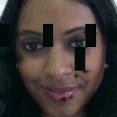
Examples of actually generated data augmentation are shown below:
| Augmentation Example 1 | Augmentation Example 2 | Augmentation Example 3 | Augmentation Example 4 |
|---|---|---|---|
 |
 |
 |
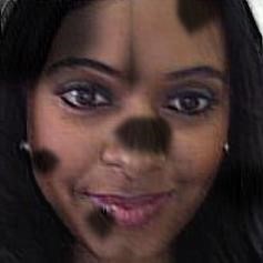 |
In the actual experiment, a total of 91,702 training images were generated, with an average of 44.85 augmented images generated per training set image.
Finetuning Based on VGGFace
On GitHub, the author rcmalli trained a face recognition model on the VGGFace dataset using Keras [3], with the following architectures:
- VGG16
- RESNET50
- SENET50
Based on these 3 network architectures, the author trained networks for face recognition using the Oxford VGGFace face data. This experiment is based on the RESNET50 architecture network model, preserving the weights before the fully connected layer, and finetuning the fully connected layer using the augmented training set images. The accuracy curves for the training set and test set during training are shown below:
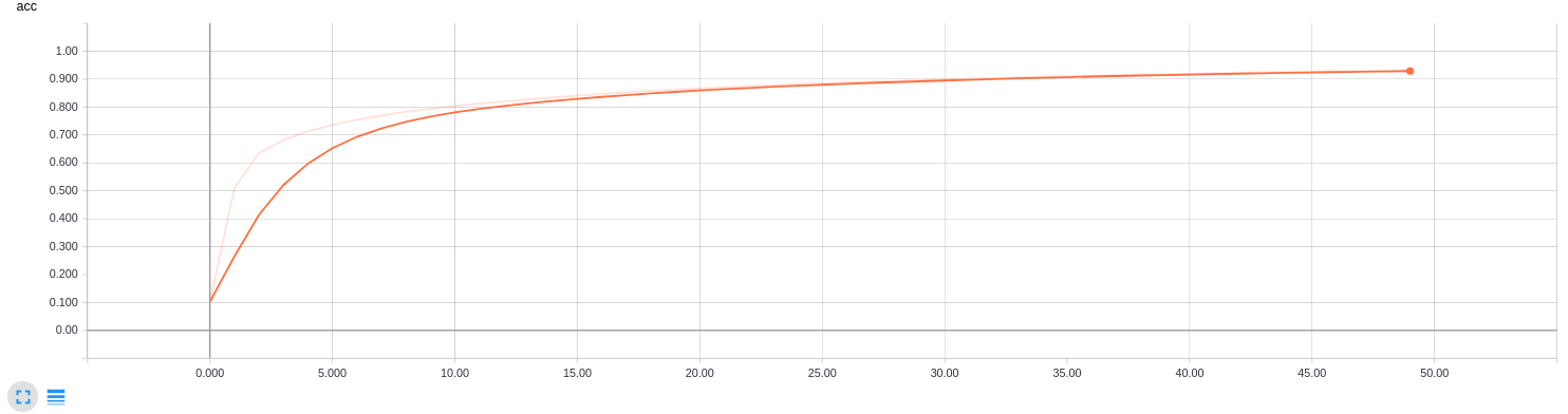
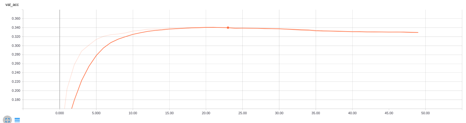
It can be seen that after 50 epochs of training, the maximum training set accuracy reached 0.9307, and the maximum test set accuracy reached 0.3375. After testing, the Top 1 accuracy was 0.3375, and the Top 5 accuracy was 0.489.
Lazy Learning Based on FaceNet
In 2015, Google researchers proposed FaceNet, which trains a network to obtain a 128-dimensional feature vector of a face, thereby obtaining the similarity between faces by computing the Euclidean distance between feature vectors.
On GitHub, the author davidsandberg trained FaceNet using the Inception ResNet v1 architecture based on VGGFace2 data [4], achieving an evaluation accuracy of 0.9965 on LFW.
The idea of Lazy Learning is to compute the distance between test samples and training set samples. Following the approach of Lazy Learning, for each test face image, we compute its similarity with all training set faces, and rank the distances from lowest to highest, thereby returning the training set face image that is most similar to the test image.
The face extraction process is shown in the figure below:
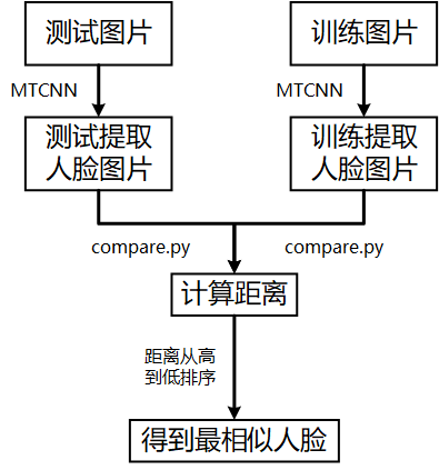
FaceNet uses MTCNN to extract the face region from the input image, then uses the author-provided compare.py to compute the similarity between two given images. During the experiment, each image in the test set needs to compute similarity with the 2,000 images in the training set. This can be sped up dramatically by pre-computing and saving the face extraction results to disk, and reading those pre-saved results when computing face distances.
An example of the final computed face distances is shown below:
0          0       1.3858
0          1       1.3257
0          2       1.5103
0          3       1.1707
0          4       1.0327
0          5       1.4050
0          6       1.5472
0          7       1.3509
0          8       1.3133
0          9       1.4988
The first column is the index of the test image, the second column is the index of the training image, and the third column is the distance between the images.
After sorting all image distances from smallest to largest and outputting their top 5 indices, the example results are as follows:
120:332,120,1534,405,356
121:121,193,1536,1252,1984
122:122,987,1165,780,1317
123:123,1077,1154,135,1222
124:550,600,124,1292,589
125:953,549,125,1981,1729
126:126,138,1820,1699,462
127:127,1003,1013,1441,325
128:201,817,1002,2,717
The first column is the test set image index, and after the ":" are the top 5 closest image indices in the training set.
After testing, using the original facenet default model, the Top 1 accuracy was 0.446, and the Top 5 accuracy was 0.6115.
FaceNet Finetuning
Previously, the original facenet model was used directly, which contains no information about these 2,000 faces. Therefore, based on the original facenet model, we re-fine-tuned using the 2,000 face images as the training set.
- Loss: softmax loss + center loss + regularization term sum; training set consists of 2,000 training images and 2,000 corresponding grayscale images. Load the facenet model trained on VGGFace for finetuning.
- Loss: triplet loss; training set consists of 2,000 training images and 8,000 corresponding augmented images. Load the facenet model trained on VGGFace for finetuning.
After obtaining the fine-tuned model, the images are classified using a KNN classifier (k=1, distance metric: Euclidean distance) following the process described above.
Ensemble Classifier
The diversity of the three base classifiers is mainly reflected in the following aspects:
- Different parameters, loss functions, and training images during fine-tuning
- Model 1: no fine-tuning
- Model 2: softmax loss + 2,000 training images and 2,000 corresponding grayscale images
- Model 3: triplet loss + 2,000 training images and 8,000 corresponding augmented images
- Different image processing methods when extracting features
- Model 1: original images processed with MTCNN
- Model 2: original images processed with both MTCNN and OpenCV
- Model 3: grayscale images processed with both MTCNN and OpenCV
The final ensemble result achieved a Top 1 accuracy of 0.6975 and a Top 5 accuracy of 0.821.
Visualization
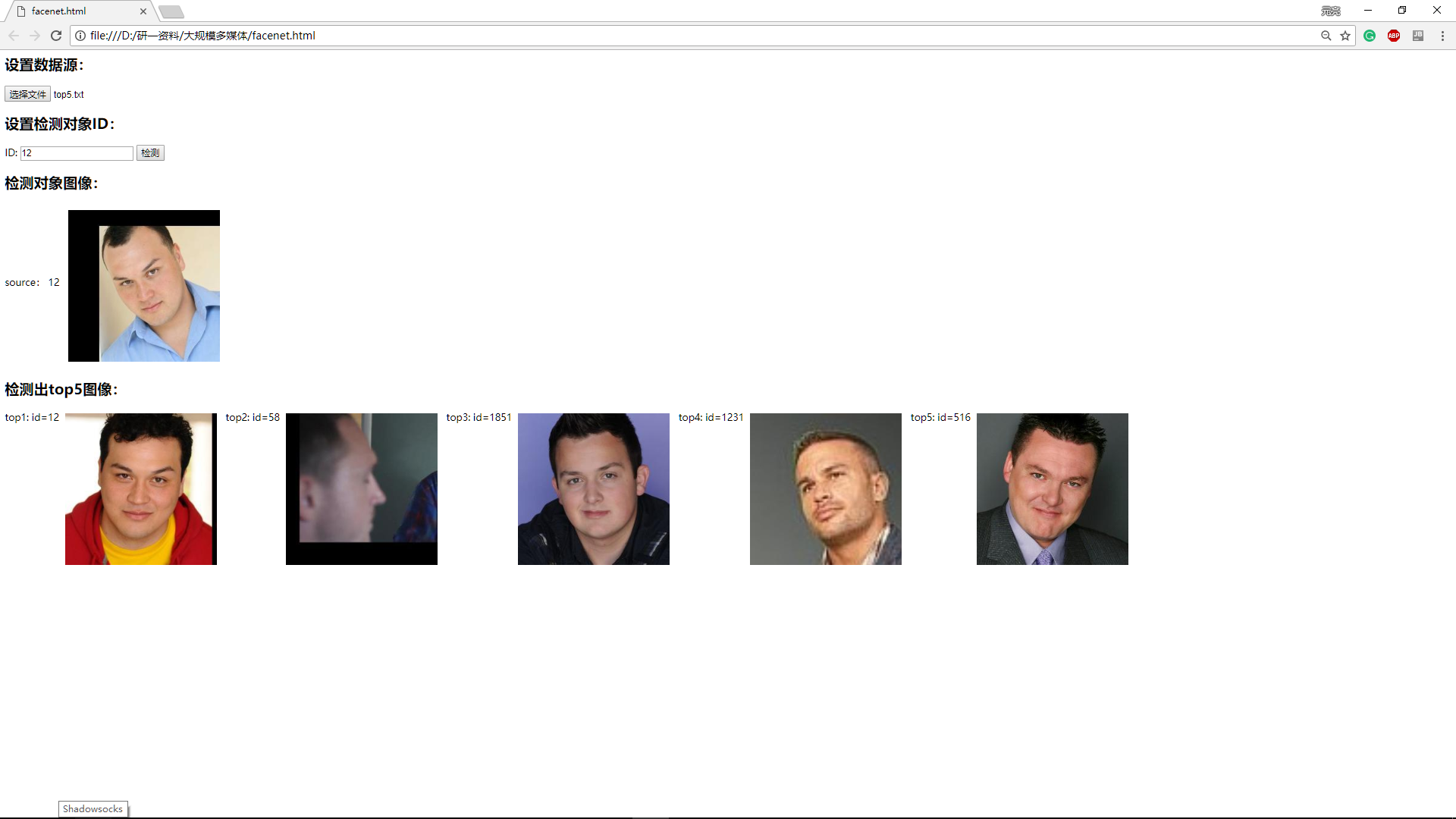
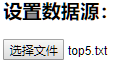
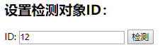
| Run the final result data from the imported model | Input the ID of the object to be detected (IDs are consistent with the given test set) |
|---|---|
 |
 |
Finally, the 5 closest face results are displayed:

Conclusion and Reflections
After testing, the Top 1 accuracy was 0.6975 and the Top 5 accuracy was 0.821.
Given time and resource constraints, potential points for improvement are as follows:
- The three face alignment methods — dlib, Haar features, and MTCNN — could be ensembled to better crop face regions from both training and test images, improving the accuracy of face comparison.
- It could be considered to extract facial features such as eyes, nose, and ears and then use neural networks for training. This would involve a substantial amount of manual data labeling work and investigation of facial feature extraction methods. Then an ensemble could be built from the classifiers trained on each facial feature, using a majority voting mechanism to match faces based on facial feature matching results, potentially achieving higher accuracy.
- Through manual analysis, it was found that the main classification errors occur when matching a person's frontal face to their profile face. Techniques such as TP-GAN could be used to convert profile face images into frontal face images.
References
[1] https://github.com/opencv/opencv/tree/master/data/haarcascades [2] https://github.com/aleju/imgaug [3] https://github.com/rcmalli/keras-vggface [4] https://github.com/davidsandberg/facenet